An Introduction to Digit Image Classification with KNN and the MNIST Dataset
November 22, 2020
Table of Contents
- Introduction
- What is the MNIST dataset?
- A Quick Review of KNN
- Digit Classification in Code and Three techniques to Improve KNN
- Summary
Introduction
In this tutorial, we introduce the MNIST dataset and show how to use K-Nearest Neighbors (KNN) to classify images of handwritten digits.
The inference problem is:
- X = an array of pixels that represent images of handwritten digits
- y = a corresponding array of labels classifying the handwritten digit as 0-9
What is MNIST dataset?
MNIST is a large dataset of handwritten images of digits collected by the National Institute of Standards and Technologies and is often used for training image processing models. The dataset contains over 60,000 images of 28x28 pixels or a total of 784 pixel values for each example. With convolution nets, error rates of < 0.25% have been achieved [1]. With KNN, error rates are between 0.5 to 5%. This guide will attempt to apply KNN to this image classification problem.
A Quick Review of KNN
KNN or K-Nearest Neighbors is a type of supervised learning that is non-parametric, requires no training, but has a high memory and inference time cost. Given the model’s high inference time cost, it is often used to develop a baseline for more complex models.
The KNN algorithm works by comparing new datasets with those the model was fitted on. The comparison is operated using a distance metric. In two dimensions, a distance metric would the length of a line between two points, or the famour Pythagorean Theorem.
If L is the distance metric and X = (x_1, x_2) are two points on a 2-D plane, then L is defined as:
In higher dimensions, the distance metric is generalized to a term called the L-norm and is written as:
When n=2, the L-norm is when we have two features X = (X1, X2) as presented above.
Once the distance metrics are calculated, the a new datapoint is classified based on the label of the nearest neighbor(s) or training data that is the closest. The k in the KNN thus represents the shortest distance between k neighbors instead of just 1 for example.
Digit Classification in Code
In this next section, KNN models are built and tested on MNIST dataset.
We’ll start off by loading the neccesary libraries. The KNN models will be built using KNeighborsClassifier from sklearn library [2].
import time
import numpy as np
import matplotlib.pyplot as plt
from sklearn.datasets import fetch_openml
from sklearn.neighbors import KNeighborsClassifier
from sklearn.metrics import confusion_matrix
from sklearn.metrics import classification_report

# Set the randomizer seed so results are the same each time.
np.random.seed(0)
Next the dataset is loaded and prepared for modeling in three ways: (1) scale down the greyscale, (2) shuffle the dataset, and (3) split into train, test, and dev. A mini_train_data and mini_train_labels dataset are created to reduce operating time in demonstrating how to build the models. In total, there are 70,000 examples or rows of data and each example contains 784 columns of pixel values that represent the image.
# Load the digit data from https://www.openml.org/d/554 or from default local location '~/scikit_learn_data/...'
X, Y = fetch_openml(name='mnist_784', return_X_y=True, cache=False)

# Rescale grayscale values to [0,1].
X = X / 255.0

# Shuffle the input: create a random permutation of the integers between 0 and the number of data points and apply this
# permutation to X and Y.
# NOTE: Each time you run this cell, you'll re-shuffle the data, resulting in a different ordering.
shuffle = np.random.permutation(np.arange(X.shape[0]))
X, Y = X[shuffle], Y[shuffle]

print('data shape: ', X.shape)
print('label shape:', Y.shape)

# Set some variables to hold test, dev, and training data.
test_data, test_labels = X[61000:], Y[61000:]
dev_data, dev_labels = X[60000:61000], Y[60000:61000]
train_data, train_labels = X[:60000], Y[:60000]
mini_train_data, mini_train_labels = X[:1000], Y[:1000]
data shape:  (70000, 784)
label shape: (70000,)
To get a sense of the dataset, the handwritten digit images are visualized with the imshow() function. Ten images are randomly choosen from each digit in the mini_train_data set. Recall that each sample contains 784 columns of pixel values or features and if reshaped to 28x28 grid, would form an image.
examples = 10
digits = 10
fig, axs = plt.subplots(nrows=digits, ncols=examples, figsize=(10, 10))
plt.rc('image', cmap='gray')

# Plots the first 10 digits from the mini_train_data set
for i in range(examples):
    for j in range(digits) :
        num_match = mini_train_data[mini_train_labels == str(j)]
        num = num_match[np.random.randint(len(num_match))]
        num_image = np.reshape(num, (28,28))

        # Plots the images of each example for each digit
        axs[j][i].imshow(num_image)
        axs[j][i].axis("off")
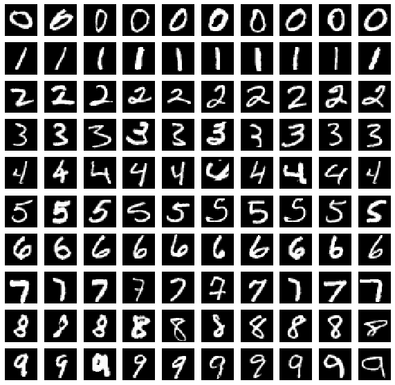
It is apparent how diverse handwritten digits can be. Sometimes zeros look like sixes, and sometimes fives look like a letter s. In the next few steps, models will be developed and we can see how they handle the handwritten numbers. Specifically, three techniques will be tested to improve the accuracy of the KNN models: examining the hyper parameter k, changing the training size, and applying an image processing technique Gaussian Blur.
The first KNN models are built around different hyper parameters k, or the number of nearest neighbors. The following script builds give KNN models, each with a different value for k. The accuracies are then stored and plotted against the number of k. It is apparent from the accuracy vs k neighbors plot that increasing the number k neighbors resulted in a loss of accuracy and overfitting. In the following examples, we will continue with k=1.
# Build KNN model
target_names = np.unique(mini_train_labels)
k_values = [1, 3, 5, 7, 9]
model_accuracy = []
for k in k_values:
    target_names = np.unique(mini_train_labels)
    model = KNeighborsClassifier(n_neighbors = k)
    model.fit(mini_train_data, mini_train_labels)
    predicted_labels = model.predict(dev_data)
    model_accuracy = classification_report(y_true=dev_labels, y_pred=predicted_labels,  # Get the accuracy for each k
                          target_names=target_names, output_dict=True)['accuracy']

# Plot results
plt.plot(k_values, model_accuracy)
plt.xlabel('k')
plt.ylabel('model accuracy')
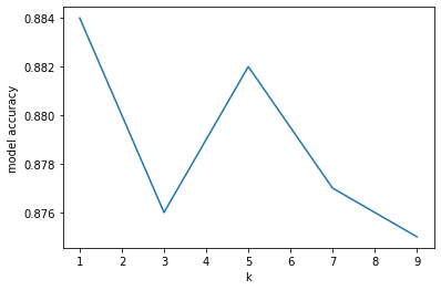
With an accuracy of 88%, its not bad! Let’s take a look at which digits KNN how difficulties with.
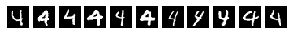
The following script grabs the confusion matrix for a KNN model where k=1. The x and y axis of the confusion matrix represents predicted digits vs labeld digits from the dev set. The diagonal of the confusion matrix represent the number of times the model was correct and the off diagonals represents where the model predicted incorrectly. The most incorrect predictions come from when a dev example was a 4 but was labeled as a 9.
# 1-Nearest Neighbor model and produce confusion matrix
model = KNeighborsClassifier(n_neighbors = 1)
model.fit(mini_train_data, mini_train_labels)
predicted_labels = model.predict(dev_data)

print("Confusion Matrix")
print(confusion_matrix(dev_labels, predicted_labels))
Confusion Matrix
[[101   0   1   0   0   0   1   1   2   0]
 [  0 116   1   0   0   0   0   0   1   0]
 [  1   4  84   2   2   0   2   4   6   1]
 [  0   2   0  84   0   6   0   2   3   0]
 [  0   0   1   0  78   0   0   2   0  11]
 [  2   0   0   1   1  77   5   0   2   0]
 [  1   2   1   0   1   2  94   0   1   0]
 [  0   1   1   0   0   0   0  96   0   4]
 [  1   5   4   3   1   3   0   1  72   4]
 [  0   1   0   0   3   2   0   7   0  82]]
To dig a bit deeper, the following script grabs the dev examples which were labled 4 and predicted as 9 by the model.
# Creates a list of pairs (dev_labels, predicted_labels)
pair_true_predicted = []
for x, y in zip(dev_labels, predicted_labels):
    pair_true_predicted.append((x, y))

# Record which index positions correspond to incorrect predictions
incorrect_prediction = []
for i in range(len(pair_true_predicted)):
    if pair_true_predicted[i] == ('4', '9'):          # Check where the model was provided '4' but predicted '9'
        incorrect_prediction.append(i)

# Initialize a plot
fig, axs = plt.subplots(nrows=1, ncols=len(incorrect_prediction), figsize=(5, 10))
print('\nExamples of 4 were predicted as 9')

# Produce a subplot of the 4s that were incorrectly predicted
i = 0
for j in incorrect_prediction:
    num_image = np.reshape(dev_data[j], (28,28))

    axs[i].imshow(num_image)
    axs[i].axis("off")
    i = i + 1
Manipulating the hyperparameter k is one way to improve the accuracy of KNN and another way is increasing the amount of training data. More training data gives the model more comparisons with the distance metric and should provide more accurate predictions. A drawback however, is that there are more computations to perform. Thus, KNN is model that requires no fitting time but a significantly computational inference time.
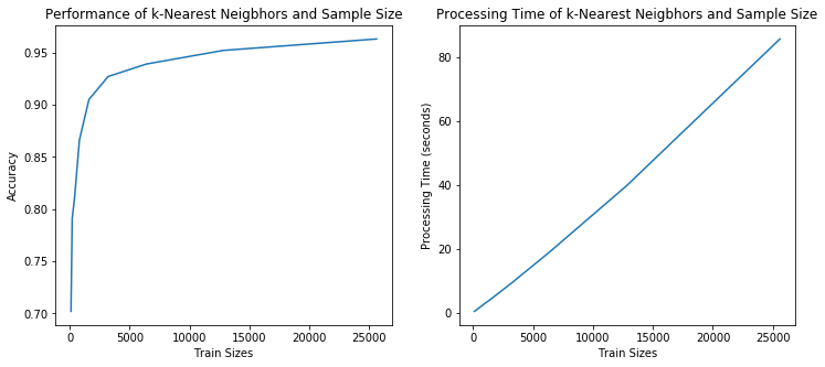
A second set of KNN models are built in the following script and explores accuracy vs training sizes from 100 to 25,600 rows of data. It also records the amount of time it takes perform inference on the dev set. From the plots, the accuracy begins to plateu at 10,000 examples while the inference time contains to increase linearly - a clear situation of diminishing returns.
# Initialize subplots and the list of train sizes
fig, (ax1, ax2) = plt.subplots(nrows=1, ncols=2, figsize=(12,5))
train_sizes = [100, 200, 400, 800, 1600, 3200, 6400, 12800, 25600]

# Build a funcion that performs 1-Nearest Neighbor for each train size
def kNN_accuracies(train_data, train_labels, dev_data, dev_labels, train_sizes):
    times = []
    accuracies = []

    for sizes in train_sizes:
        t1_start = time.process_time()                            # Start recording process time
        shuffle = np.random.permutation(np.arange(sizes))         # Shuffle for random sampling

        # 1-Nearest Neighbor
        target_names = np.unique(train_labels)
        model = KNeighborsClassifier(n_neighbors = 1)
        model.fit(train_data[shuffle], train_labels[shuffle])
        predicted_labels = model.predict(dev_data)

        # Get accuracies for each train size
        accuracies.append(classification_report(y_true=dev_labels, y_pred=predicted_labels,
                                                target_names=target_names, output_dict=True)['accuracy'])

        t1_stop = time.process_time()                              # End recording process time
        times.append(t1_stop-t1_start)                             # Calculate elapse process time

    return(times, accuracies)

# Store the accuracies and process times for each train size
times, accuracies = kNN_accuracies(train_data, train_labels, dev_data, dev_labels, train_sizes)

# Plots Accuracies vs Train Sizes
ax1.plot(train_sizes, accuracies)
ax1.set_xlabel('Train Sizes')
ax1.set_ylabel('Accuracy')
ax1.set_title('Performance of k-Nearest Neigbhors and Sample Size')

# Plots Processing Time vs Train Sizes
ax2.plot(train_sizes, times)
ax2.set_xlabel('Train Sizes')
ax2.set_ylabel('Processing Time (seconds)')
ax2.set_title('Processing Time of k-Nearest Neigbhors and Sample Size')
plt.show
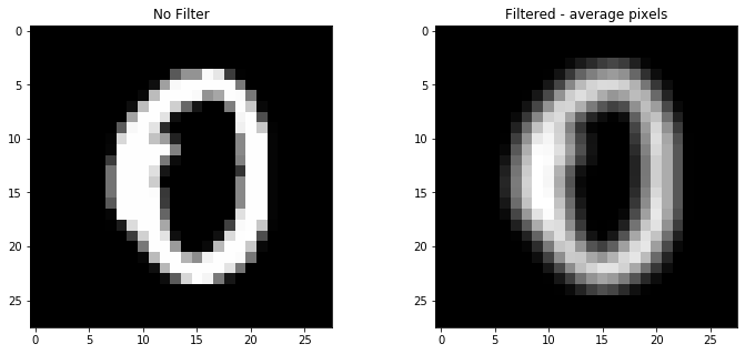
Since high computational inference times are often inhibitive in practice, the last technique we will apply to improve accuracy is Gaussian Blur. Gaussian Blue is an common image processing technique that smooths an image by blurring. The idea is that a value of a particular pixel is a weighted average of the pixels around it. The weight of surrounding pixels on the particular pixel is determined by the Gaussian function (mean and variance). Ultimately, the technique reduces the complexity of the images and generalizes the model.
In the third set of KNN models, the script below builts a function called gaussian_blur which averages the 8 neighboring pixels and assigns that value to the particular pixel. Two KNN models are then produced, one for the raw dataset and another for the transformed train dataset. From the results, we can see the the accuracy of the now has now increased to 91%. Thus we were able improve accuracy despite reducing complexity.
def gaussian_blur(data):
    '''
    data = a 2D np.array
    '''

    # Initialize new array to accept the filtered data
    examples = data.shape[0]
    pixels = data.shape[1]
    g_data = np.zeros([examples, pixels])

    # Iterate through every row in the dataset and calculate the average pixel value
    for k in range(examples):
        num_image = np.reshape(data[k], (28,28))    # Each row of 784 pixels is converted to 28x28

        new_num_image = np.zeros([28, 28])          # Temporarily store new pixel values

        # Index values are used to find the 8 surrouding pixels around center pixel (i,j)
        for i in range(1, 27):                      # Index values range from (1,27) to ignore edges
            for j in range(1, 27):
                new_num_image[i, j] = 1/9*np.sum([num_image[i, j], num_image[i, j-1], num_image[i,j+1],
                                             num_image[i-1, j-1], num_image[i-1, j], num_image[i-1, j+1],
                                             num_image[i+1, j-1], num_image[i+1, j], num_image[i+1, j+1]])

        # Store the filtered pixels into the new array
        g_data[k] = new_num_image.reshape(pixels)

    return g_data

# Example of Gaussian Blur on mini_train_data set
fig, (ax1, ax2) = plt.subplots(nrows=1, ncols=2, figsize=(12,5))

gb_mini_train_data = gaussian_blur(mini_train_data)
gb_dev_data = gaussian_blur(dev_data)

ax1.imshow(mini_train_data[0].reshape(28,28))
ax1.set_title("No Filter")

ax2.imshow(gb_mini_train_data[0].reshape(28, 28))
ax2.set_title("Filtered - average pixels")
plt.show

# Peform kNN for the 2 scenarios for k=1

KNN_0 = KNeighborsClassifier(n_neighbors = 1)
model_0 = KNN_0.fit(mini_train_data, mini_train_labels)
accuracy_0 = model_0.score(dev_data, dev_labels)

KNN_1 = KNeighborsClassifier(n_neighbors = 1)
model_1 = KNN_1.fit(gb_mini_train_data, mini_train_labels)
accuracy_1 = model_1.score(dev_data, dev_labels)

print("No Filter Train, No Filter Dev: %0.2f" %accuracy_0)
print("Filter Train, No Filter Dev: %0.2f" %accuracy_1)
No Filter Train, No Filter Dev: 0.88
Filter Train, No Filter Dev: 0.91
Summary
In this guide, we looked at the MNIST handwritten digit dataset and how we could apply a K-Nearest Neighbors classification from sklearn library to classify the digit images. Out of the box, KNN produced an accuracy of 88% with k=1 and increasing k did not improve model performance. We increased the training set size for the KNN model and saw increased accuracy but it was at the cost of a high computational inference time. Instead, applying an image processing technique called Gaussian Blur generalized the model and improved model accuracy to 91% with little cost.